
In 2013, 90% of businesses reported using Microsoft Excel in their business operations.
In 2016, 1 in 5 companies report using Excel as their primary mode of communicating data internally.
However, the world is catching up and Excel is wandering into a future of SaaS apps and automation. If you have Excel deep within the structures of your business, this article will show you two key things:
- How to get the most out of Excel. Learn how to do more than the basic calculations and how to bring automation into your Excel operations.
- The other automation tools on the market which you can begin to integrate into your operations as you move forward.
What we’re going to do is lay out a series of steps by which you can get more from Excel. We’re going to start off super simple with our Excel for dummies, and move gradually up to complex tasks which can really demonstrate the power of Excel.
Are you ready?
Good.
Firstly, let’s look at what Excel is usually employed for.
Excel for Dummies
Every company’s use case for Excel may be subtly different. Nevertheless, there are a couple of core functions Excel is often given the responsibility of handling.
Scheduling
Many companies use Excel for defining working hours and timesheets. This can often be used to manage payroll for companies which pay via hourly employment, or defining contractor relationships. Excel is often also used to schedule meetings or availability of meeting rooms and other workspaces. Traditionally, this would require an individual working in an administrative capacity to be responsible for managing these spreadsheets. With Microsoft 365 and other improved services over the years, much of this work has been shifted into cloud-based provision.
Tip 1: To make your scheduling work more clearly, use color coding on your spreadsheet with a neat key on the side. Each cell can be given a different background color and you can enhance the borders on headers to make the table easier to understand at a glance. You can do this easily by selecting your data, right clicking, and selecting Table. Excel will automatically make it look pretty, then you can customize.

Or, instead of making your own timesheets, why not start off with templates made by others? Time Doctor’s timesheet templates give you a host of different structures to choose from, and you can get them in other formats too. Choose from weekly, fortnightly, or monthly!
Accounting reporting
Excel’s spreadsheet and basic calculation functionality have historically made it an essential feature of accounting departments. It’s very easy to record data and manage that data, adding and subtracting against columns. Through being able to easily generate reports and charts, Excel provided and continues to provide a way to both manage accounting tasks and to compile and present accounting performance in easy to use ways.
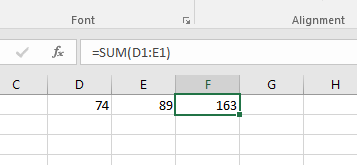
Tip 2: You can do simple calculations within Excel using commands like SUM. To run these commands, select the cell you want the result to appear in and type “=SUM” followed by brackets with the number of the first cell in the column you want to add up. Then add a colon to separate it from the last cell in the column you wish to add together and close the brackets. Press enter and Excel will add that range up for you.
Tracking performance
If you wish to understand your company’s operations by numbers, Excel’s spreadsheet view provides an intuitive way to record all relevant data and see how certain elements relate to others. You can track production costs versus sales performance and map that against operating costs with ease. From this base, you can use Excel to draw projections and spot downstream problems in your business operations. Excel has been used in boardrooms across the world to understand company direction.
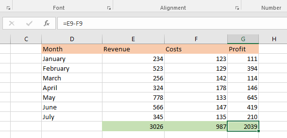
Tip 3: To calculate a series of cells you can do simple commands. If you have a column for revenue and one for costs, you can calculate profits by selecting the cell you want this to appear in and typing “=” followed by the number for the revenue-total cell, the minus sign, and then the number for the costs-total cell. Press enter and Excel does the calculation for you. If you used the SUM formula above to calculate those totals, then any number which changes in the revenue or costs columns will make Excel recalculate the profit total.
Customer information
As you gather new customers, you need to keep track of them and the different variables pertaining to their relationship with your company. Excel is often used to record this customer information, with the ability to easily search for specific customers within this database making it a simple way to record and track individual contracts. With the ability to create new columns as and when they are needed, the spreadsheet layout makes the data contained highly malleable.
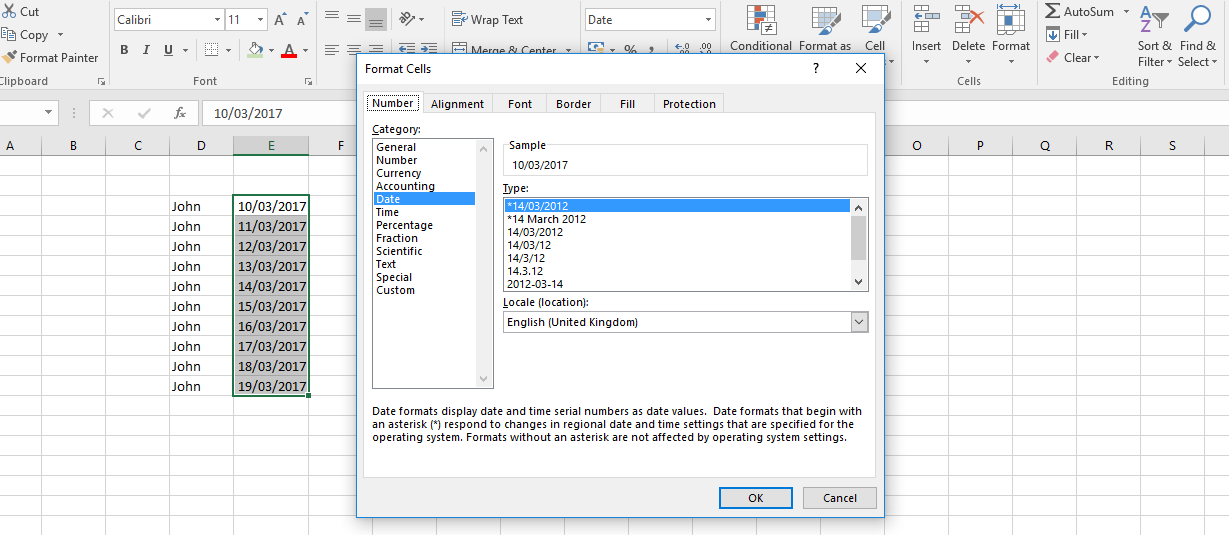
Tip 4 + 5: When compiling data on customers, you may record the date they joined you or the date they purchased your product. When you enter a date into Excel, it automatically understands you are using dates and formats the column accordingly. However, you can alter the way a column is formatted by right clicking on the column and selecting “Format cells”. You can also change the way these dates are sorted by clicking on Sort & Filter in the top right of your screen.
There are countless use cases for Excel and the above are simply the most common broad categories. Even if you are using Excel in a simple way, you can improve your processes and efficiency through applying a few simple tips and tricks.
Let’s have a look at some of the basic steps to improving your Excel usage.
Tips and tricks to get the most out of Excel
I’m going to assume you know how to type a number into a box. I’m also going to assume you already have the need to have lots of numbers in boxes, but maybe need to be able to more easily interpret those numbers or run calculations automatically.
Here are the 5 tips we’ll cover in depth:
- SUMIFS Formulas
- VLOOKUP Formulas
- INDEX+MATCH Formulas
- IF Formula
- Nesting Formulas
Tip 6: SUMIFS Formulas
Imagine you have two products which you sell across three different regions and you have two defined customer types. What you want to know is how many of a particular product in a particular region you sold to a particular customer type.
This isn’t the easiest thing to do if you don’t know how to make Excel do the analysis for you. This is where the SUMIFS command comes in. SUM is about adding stuff, and IF is about controlling for variables. So, SUMIFS is about adding certain stuff together providing certain parameters are met.
It looks a little something like this:
=SUMIFS(sales, regions, “A”, products, “B”, customer types, “C”)
The first value above is what we want to add together. The second value is us defining a dataset (the region), with the third value being the variable we want to use from that dataset (a specific region). The fourth and fifth are paired together in the same way. As are the sixth and seventh.
It might look like this:
=SUMIFS(A1:A100, B1:B100, “South”, C1:C100, “Chocolate bunnies”, D1:D100, “Commercial outlets)
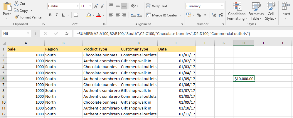
This scans through the sales data in column A and pulls out all the information which matches the parameters you’ve defined in the rest of the formula. It then adds these figures up and presents you with the total.
If we say that the sales figures are total dollar sale amounts for each purchase, then the amount of chocolate bunnies sold to commercial outlets in the south would come out as $10,000 – or whatever the actual sales figures would be.
This turns a complex task into a simple calculation which can be completed rapidly, saving you time and keeping you focused on the important things.
Tip 7: VLOOKUP Formulas
The best way to imagine the VLOOKUP is a search engine which shoots back the answer to you. Like any good search engine, it’s all about defining what it is you’re looking for.
If you have a large table with a number of different columns and you know one piece of data (“datum” – to save you the effort of reminding me in the comments) and you want to find out about another bit of information related to that data, you can use the VLOOKUP.
Let’s pretend we have a sheet which contains, amongst other things, customer names and customer IDs. What we want to do is enter the customer ID and have Excel shoot the customer name right back at us. We’ll assume the customer ID is 12345 and the column for customer names is the second column in a table of customers which spans cells A1 to D20.
It should look something like this:
=VLOOKUP(12345, A1:D20, 2, 0)
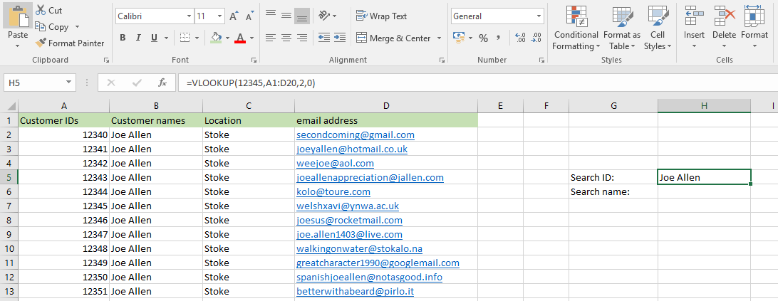
Which means we’re performing the lookup on the customer ID within the table of customers, and then pulling out its corresponding value recorded in column number 2, and we want an exact match; “0” means “false” – the value “1” would mean “true” and would give us an approximate match.
In the defined table – A1:D20 – the VLOOKUP will automatically search within the first column for your search term, in this case the customer ID. When it finds it, it will then look at the value next to it in the second column, in this case column B.
Excel will then return that value to you. Like a search engine, but for your spreadsheet.
It’s important to be aware, that if your table is defined as D1:F20, for example, column number 2 would be column E, because that is the second column within your defined range.
Also, always use the column your search term is in as the first column in your defined range. The VLOOKUP automatically searches this column for your search term anyway, so it saves headaches for you to just follow along. If your customer ID is in column F and the name is in column G, don’t use A1:G20, use F1:G20 as your defined range. It just makes things a little easier.
Tip 8: INDEX+MATCH Formulas
The problem with VLOOKUP is that it only searches in the left-hand column.
The painfully obvious limitation of this is that it makes it difficult to find things which are stored to the left of the term you are searching for. So, how do we fix this?
This is where we have to use the INDEX+MATCH approach.
This works by first stating what you want to find and then defining what corresponding information Excel can use to find it.
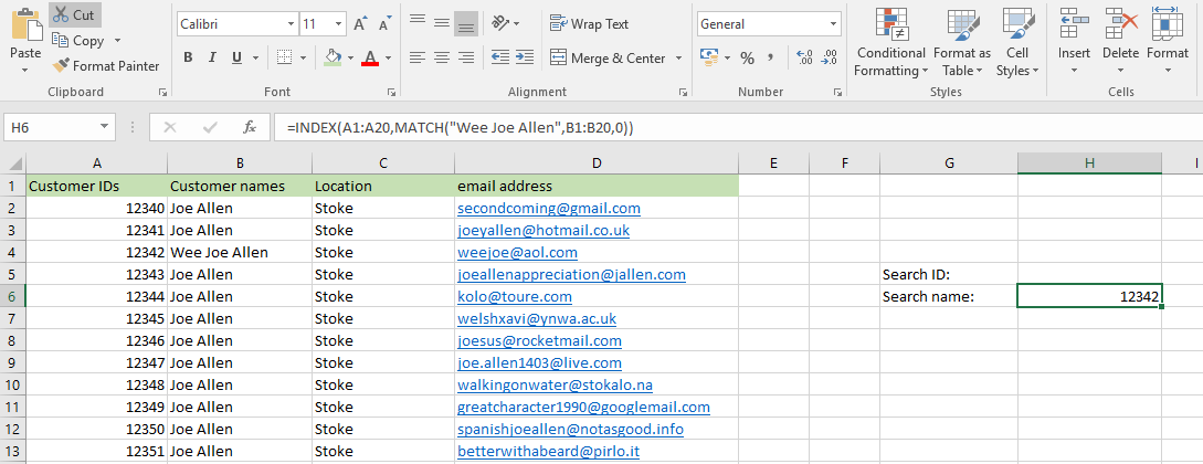
Let’s say we have the name of a customer, but we want to find their customer ID. The reverse of the example given in the VLOOKUP explanation above. This means the customer names are in B column between cells 1 and 20, and the customer IDs are in A column between 1 and 20.
First, we have to tell Excel what we want to find:
=INDEX(A1:A20)
Now we need to insert the MATCH command into that formula. It slots in nicely before the end of the brackets separated by a comma and with its own set of brackets after it:
=INDEX(A1:A20, MATCH())
Inside those second brackets we put the parameters for the item we know we’re searching against – the name of the customer, its location, and whether the column is sorted (0 means false, 1 means true):
=INDEX(A1:20, MATCH(“Wee Joe Allen”, B1:B20, 0))
The above formula should search the B column for the customer Wee Joe Allen and return to us the corresponding figure from the A column – Wee Joe’s customer ID.
Simples, no?
Tip 9: IF Formula
You can use IF formulas in loads of different ways, but we’ll give you a pretty simple scenario to get you started.
Imagine you have 10 employees and they all earn $3,000 per month. You’ve told them time and time again to subscribe to the Process Street blog. You’ve decided that you’re going to incentivize them further by giving a raise to all the employees who have subscribed to the blog. You’re going to give them all a raise, because you’re nice like that, but you’re going to give a bigger raise to subscribers.
A 10% raise to blog subscribers and a 5% raise to the rest.
You might have lots of important columns detailing your employees’ information but for us there are two columns of importance.
The first column we care about is the column which lists their monthly wage. A column of 10 where every cell contains the figure “3000”. Let’s say this column is located E2:E11.
The second column you create is designed to record whether or not the employee is subscribed to the Process Street blog. Let’s say this column is F2:F11. Against each employee, you give a score of 0 or 1. If they are subscribed to the blog, they receive the score “1” which means the statement is true.
What we can do now is build the basic formula in the next cell along; G1. The formula will look something like this:
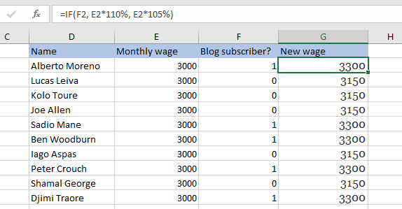
=IF(F2, E2*110%, E2*105%)
Let’s look at what this means.
F2 is where you stated your true or false expression: 0 or 1. E2 is the original wage they were receiving. So, of the three parts to the above formula, part one asks whether the statement is true or false, part two defines what happens if the statement is true, and part three defines what happens if the statement is false.
So if E2 contains the value “3000”, F2 contains the value “1”, then Excel will calculate that G2 will contain the value “3300”.
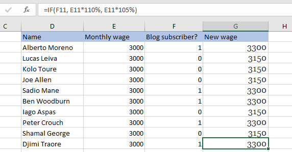
Tip 10: Now you select the G2 cell and click on the little blue square which appears on the bottom right-hand corner of the cell. Drag that down the page to G11 and Excel will calculate all the figures for all the other cells automatically.
If you now click on G11, you should see the formula:
=IF(F11, E11*110%, E11*105%)
… automatically generated without you having to type it out.
Tip 11: Nesting Formulas
Sometimes you’re faced with something a little more complex than a true or false value can define. Maybe you have to deal with multiple different variables?
Do not fear.
For these kinds of scenarios, we can put formulas inside formulas and work out more complex things.
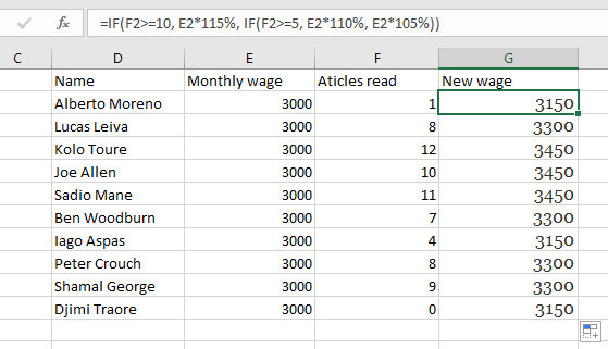
Let’s take the same employee raise scenario we used above. However, this time you want to give a raise to someone based on how many Process Street articles they have read each month. We pump out a minimum of 12 articles a month and you want your staff to read every last one of them.
You’ve decided that you’re going to hand out a 15% rise for anyone who has read over 10, a 10% rise for anyone who has read over 5, and a 5% rise for everyone else because you know the cost of living is rising and Terry just had another child, bless him.
How do we do this?
Imagine your data is laid out similarly to before. If you’re following along in Excel, list the number of Process Street articles each employee has read that month in column F, and we’re going to do our calculations in cell 2 of column G again.
In the last IF formulas, the structure was:
IF condition, result if positive, result if negative.
Part 1, part 2, part 3.
We’re going to do that again but this time we’re creating two IF statements, with the second one nestled inside the first. This time the part 1 will be whether the number of articles is above 10, and the result if positive will be the appropriate 15% raise. However, we don’t need to define a normal negative result – this time, if the result is negative we will run a second IF formula. If the second IF formula is positive the employee gets a 10% raise and if it is negative they receive a 5% raise.
Let’s write it out in plain terms below:
IF greater than or equal to 10 articles per month, if positive result times wage by 115%, if negative result run IF(greater than or equal to 5 articles per month, if positive result times wage by 110%, if negative result times wage by 105%)
When we put all that together in an actual formula, it’s going to look like this:
=IF(F2>=10, E2*115%, IF(F2>=5, E2*110%, E2*105%))
Then simply grab that little blue guy at the bottom of your selected cell and drag him down to the bottom of your employees-list to calculate the rest.
Extra useful commands and symbols
Tip 12: In the above examples, even though we made the calculations in K1 with reference to J1 and I1, once we had pulled the formula down to K10 the formula was pulling its data from J10 and I10. If you don’t want that to happen, you can lock a formula to a particular cell by using the dollar sign.
If we had used $J$1 or $I$1 the formulas we created as we dragged our calculations down the cells in the K column would have stayed attached to the original cells.
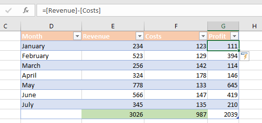
Tip 13: You can create a defined table within Excel by highlighting all the cells you want to include in your table and clicking on Table on the ribbon. Then you can format your table by clicking on any of the cells within the table and selecting “Format as Table”.
Tip 14: To make your life easier for yourself, you can name your table in the design tab. This allows you to start writing formulas which contain words rather than strings of numbers. If you name your table Financials and have a column called Revenue and another called Costs, you could work out profit by typing:
=Financials[Revenue] - Financials[Costs]
The table name is presented in plain writing with the column titles inside square brackets. Once it has been calculated, Excel will portray it in the easiest way to understand:
=[Revenue]-[Costs]
Tip 15: The ampersand symbol can be used to combine two text values. If you have one cell which has the text “David Moyes” and another which says “football genius” then you could use the formula:
=“David Moyes” & “football genius”
And you would get the result:
David Moyes football genius
Tip 16: Using the equal to / greater than kinds of commands always works with Boolean logic. This is a fancy way of saying they provide True or False outputs. A nice example of how they can be used was our Nested formula in the section above.
2<1 will result in False
1<2 will result in True
2>=1 will result in True
1>=2 will result in False
Tip 17: If you want to refer to an inline array of values, you can use the squiggly brackets. For example:
{1,2,3,4,5,6} refers to the list of values 1,2,3,4,5
Tip 18: If you want to count all the words beginning with the letter “a” in column B, you can easily do this by employing the asterisk symbol in a COUNTIF statement. Example:
=COUNTIF(B1:B100, “a*”)
Tip 19: Another neat COUNTIF trick is for finding phone numbers. If you’re an international company and you have the phone numbers of loads of clients with their country codes, you can search for the country code:
=COUNTIF(C1:C100, “44*”)
If your phone numbers are stored in column C, that should return all British phone numbers in the defined range.
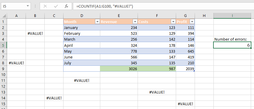
Tip 20: If you’re working with a massive sheet of data with loads of interconnected formulas, sometimes things go wrong. Don’t worry, the handy COUNTIF can tell you whenever something has popped. Lets imagine you have 100 rows of data.
Simply choose a cell to monitor the rest of your sheet and enter the formula:
=COUNTIF(A1:G100, “#VALUE!”)
This will count how many times the error code pops up in your spreadsheet across the first 100 rows. So, if you want to check nothing is broken, you can simply look at this one cell instead of analyzing your entire sheet.
Tip 21: Another COUNTIF! This time let’s assume you have a big list of cities where your customers are located. You also have a handy key on the side which tells you how many times each of your 5 target cities – where you want to expand – show up in the list.
The 5 cities are recorded in column X. London is one of them; located in X1.
In cell Y1, you want to record how many times London appeared in the list of cities of your customers: G1:G100. The list is categorized by how much they spend in descending order and you only care about the top 100 biggest spending customers, not the whole column.
Here’s your formula:
=COUNTIF($G$1:$G$100, Y1)
Or equally:
=COUNTIF($G$1:$G$100, “London”)
Build out automations with macros and add-ins
A further way to expand your Excel capabilities is to delve deeper into the complex side of what the program is capable of.
The programming language which works within Excel is Microsoft’s Visual Basic. This allows you to write more detailed code to determine how your Excel sheet functions. Building macros is the first step on that journey.
The best way to imagine a macro is to think of it as Javascript within HTML. Javascript is capable of manipulating the HTML you find on a webpage and macros do the same thing to the documents they’re embedded into.
There’s a wealth of different things you can do with macros, including:
- Applying style and formatting
- Manipulating data and text
- Communicating with other data sources (databases, text files, etc)
- Creating entirely new documents.
- All of the above in any order or combination
You can create a basic macro without any need to code by navigating to the View tab on your ribbon. On the furthest right-hand option, you’ll see a big button for Macros.
If you click the Record Macros option then you can name your Macro and begin the creation. Excel will now monitor what you do in the spreadsheet until you click to stop recording, and Excel will remember the series of steps you performed.
You can manipulate your data using formulas and apply formatting to your cells to make them look pretty – taking a series of basic numbers and turning them into a fully calculated table. Excel has watched the steps you took to achieve this and has remembered them. By saving this as a macro, you can automatically run all those steps again in an automated fashion on new data in future.
In short, you created and defined a process which you want Excel to follow, and named it. When you want to run that process on cells in the future, you can easily instruct Excel to do so.
Once you’ve stopped your recording, delete the data in the sheet and save the document in a macro-enabled format, like below:

Congratulations! You’ve made a macro.
To use this macro in future, import the data you want to manipulate into your spreadsheet and click Macros on the right-hand side of your ribbon. You’ll see the option for View Macros. Clicking this will show you all available macros and you can choose the one you need. Then click Run and watch Excel work on your document for you, making all the changes you defined when you set up your macro, to begin with.
A further step to boost the functionalities of Excel is to include add-ins. These are external programs which you can integrate into Excel to improve its functionality. Google Sheets makes use of a huge library of add-ins to supplement its more lightweight core functionalities.
Here are some Excel add-ins worth checking out:
- ASAP Utilities: The most popular add-in for Excel which provides a further +300 added functionalities.
- AbleBits Utility Pack: Provides a number of useful features including merging Excel worksheets and more.
- Ribbon Commander: For the expert user, this add-in lets you manipulate your ribbon and create your own add-ins.
- XL Tools Add-In: Add productivity tools and improved version management into your Excel usage.
- PivotalPal Add-in: This one focuses on pivot tables and provides many options for how to get the most from your tables.
Bring in extra tools to automate what Excel can’t
To really bring the best of out Excel, we should look to see how it can work with other tools outside of itself. We want to easily be able to pull data from other areas into Excel and launch things on other platforms from Excel. Having this range of features allows us to automate tasks simply and easily.
Zapier
The big boy of third party automation tools, Zapier connects with over 750 different webapps and allows them to speak to one another, triggering actions in one webapp from a different webapps.
When you connect two platforms via Zapier, you’re creating a “zap”. This zap fires the information back and forth as you’ve defined it. You don’t need to code and it only takes a few moments to set a zap up.
Zapier integrates with Excel and provides a host of different potential use cases. Check out the image below:
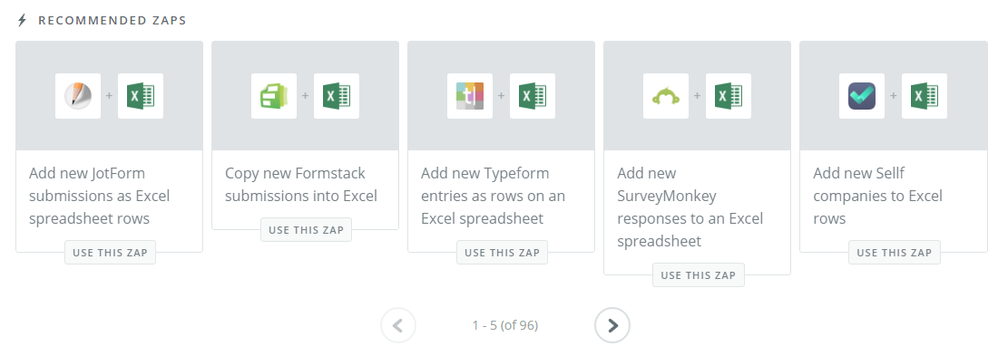
Do you see that at the bottom? Zaps 1-5 of 96. What that doesn’t include is the extra things you can achieve by setting up multi-step zaps.
The future is here and it’s automated.
Process Street
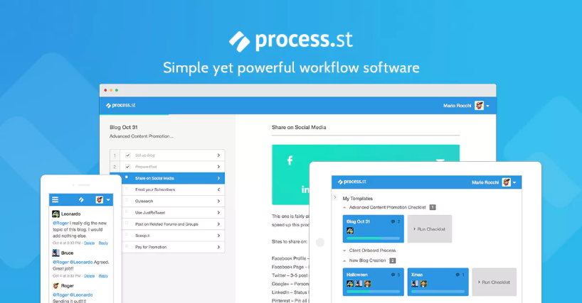
With Process Street, you can launch checklists from a library of premade or custom templates. These checklists help you define your processes and workflows in order to improve the functioning of your business.
While Excel automates your calculations for you, Process Street can automate much of your managerial and oversight responsibilities. Running a process for an employee provides them with clear and easy to follow instructions and then logs the progress they’ve made.
Using Zapier, you can connect Process Street to Excel and smooth out the workflows within your business.
Flow
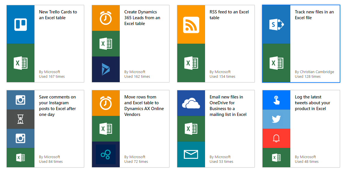
As great as Zapier is, Excel is a Microsoft product. It wouldn’t make sense to avoid mentioning Microsoft’s new product Flow, which is engineered to take on Zapier within the third-party automation market.
Flow is neatly synced up to all the Microsoft services and contains nearly 100 extra integrations too.
As Flow is a new product, expect the number of available integrations to rocket as time moves forward. Look at the image above to see the broad range of use cases Flow’s automations system provides for Excel.
And those few are only a sample. Keep an eye on Flow.
Make the most out of Excel and automate your workflows
Now that you’ve read through this article, I’m hoping you feel a little more comfortable around Excel. No longer is this Excel for dummies, but Excel for seasoned data analysts!
We’ve covered the basics, looked in depth and some harder bits, and covered a range of extra tips and tricks too.
The best way to learn more about Excel is to start putting these techniques into practice. Try to set up a sheet of data which contains multiple complex formulas and then when you’ve got it figured out, record the creation process as a macro. You’ll see how quickly you can go from an excel newbie to a power user.
Before you know it, you’ll be writing in Visual Basic and having water cooler discussions about the virtues of csv files.
Most importantly, you’ll cut out all the time wasted on manually analyzing data.
What did you find most useful from the article? What Excel use cases do you have to deal with on a day to day basis?


