

Simple as it may be, Little’s law is an incredibly powerful tool in the arsenal of almost any team. From performing back-of-the-napkin calculations to showing the performance of a system over time, this formula is one of the key building blocks to running an efficient business.
Without Little’s law, Lean and Kanban wouldn’t exist, and key elements of America’s nuclear deterrence would be left up to chance.
After all, you can’t fly B-2 stealth bombers into action if they’re all under maintenance due to bad queue management.
So stick around, because today I’ll run through what Little’s law is, how it can be applied in your own business, team, and business processes, and what elements you need to be wary of in order for it to work.
I’ll also be talking about everything from manufacturing to making chairs, to what Google and Facebook’s growth focus is, to how the stealth bomber maintenance schedule was created. Little’s law is just that useful and widespread; if you have a process with some sort of queue in it, this is by far the easiest and most consistent way to perform a rough analysis and see what’s going wrong.
Let’s get started!
Little’s law explained
Put simply, Little’s law is an equation showing that the average number of customers in a queueing system is equal to their average arrival rate multiplied by the average amount of time they spend in the system. In other words:
“No. items in the queue” = “arrival rate” x “average time spent in the queue“
While it’s a very simple calculation, the power of Little’s law comes in the way that it can be used and the fact that it relies on very few consistent elements in order to remain true.
However, before we get to the details I need to go over a few basics first. Namely, you need to know what a queueing system is, the actual formula, how it was created (trust me, the context is useful), and for good measure I’ll throw in an example to help wrap your head around the whole thing.
Little’s law applies to queueing systems
First up, Little’s law only applies to “queueing systems”. These are systems which work has to enter and leave – the work never ends (through either completion or being dropped) while inside them.

Think of a queue. When you line up, the point is never to queue. You enter the queue, spend time going through the process of queuing, and then when you’re at the front of the line you move on to whatever you were waiting in line for.
Another way to think about it is a production line. Sure, work is being done in terms of assembling items, but ultimately resources enter the production queue, spend time having work performed on them, and then leave for the next step.
The work being done while in the queue doesn’t matter (at least in terms of applying Little’s law), so much as consistently assessing just a single queue. As long as you isolate one system (or a sub-system), you can apply the law.
There are a couple of elements which need to remain consistent (which I’ll get to later), but this is why Little’s law is so widely applicable. Literally any queueing system can be assessed using this, as the actual item, work being done, or purpose of the queue doesn’t matter.
Little’s law formula
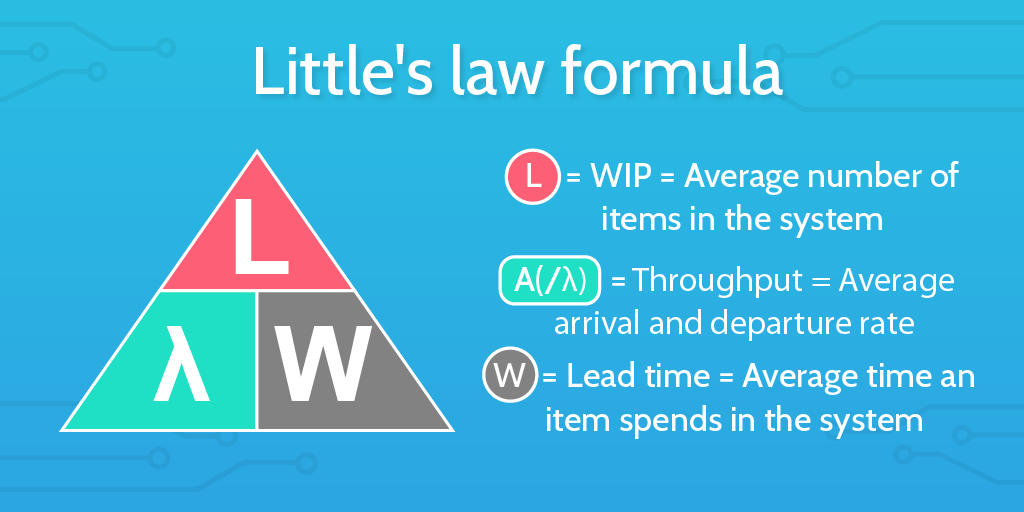
As I’ve already mentioned, the Little’s law formula is incredibly simple:
L = A x W
In this formula, “L” stands for the number of items inside the queueing system you’re examining. This is also known as “WIP”, as in, the items that are a “work in progress”, and can be pretty much any whole number.
“A” represents the arrival rate and departure rate of items in and out of the business system. This is also sometimes known as “throughput” or “the amount of an item passing into and/or out of a system”, and is sometimes represented as lambda, or “λ”.
The arrival rate is a little confusing at first, but the key to remember is that it will usually be a fraction. This is because you’re measuring the rate at which items enter/depart from the system, rather than the number of items or the time between new arrivals. As such, “A” is always expressed as a fraction showing “one item ever X units of time”, or:
A = (1 item) / (unit of time)
For example, if a new item enters your queue every twenty minutes, your arrival rate is not 20, but instead 1/20.
Finally, “W” is the average amount of time an item spends in your queueing system. This is also known as “lead time” and can also be any unit of time. The only confusing part of this element is that the unit needs to be the same as the one you used for “A” – if you measured the arrival rate in days, then “W” will also be measured in days, and so on.
So, in full English, the law becomes:
Number of items in the system = (the rate items enter and leave the system) x (the average amount of time items spend in the system)
The formula can also be changed to make any of the three elements the focus. The three possible variations are therefore:
- L = A x W
- A = L / W
- W = L / A
The history and traditional meaning

The law itself is named after John Little – an MIT professor who first mathematically proved the law in 1961. The law existed beforehand, but until Little there wasn’t a set mathematical definition of it or proof for its validity.
Little defined the law while doing operations research on traffic control signals, hence the basis of it as a way to analyze queueing systems.
Little’s law example
B-2 bombers (stealth bombers to you and me) are a vital part of nuclear deterrence. While there aren’t many (20 to be exact), these need to be in prime condition and ready to use at a moment’s notice, but also log regular flight hours and be available to train pilots or run general tests.
Unfortunately, these complex aircraft have to undergo extensive maintenance after a set amount of flight hours (and, of course, after incurring damage) in order to maintain their stealth status. This maintenance could take anywhere from 18 to 45 days, and thus resulted in a delicate balancing act between use and maintenance.

It was obvious that the maintenance process needed to be improved and regulated, but the target time wasn’t clear enough to use to introduce process improvement just yet, and that’s where Little’s law came in.
The item they needed to calculate was the ideal lead time (the time spent in maintenance), and so the formula used was:
W = L / A
Through flight schedule analysis, it was calculated that three B-2 bombers would be under maintenance at any given time. The rate at which bombers entered maintenance was also calculated to be roughly every 7 days. So:
- L = number of items in WIP (maintenance) = 3
- A = arrival/departure rate = 1 every 7 days = 1/7 days
- W = the average amount of time spent in maintenance = ???
Put into our formula, this leaves us with:
- W = L / A = 3 / (1/7 days)
- W = 3 / (1/7 days)
- W = 21 days
Therefore, the target lead time for B-2 bomber maintenance needed to be 21 days in order to meet the demands of both available aircraft and the regular flight schedules.

How to put it in action
While the equation is simple, the power of using this law comes in its myriad of uses. Heck, it even formed the basis for lean and Kanban through showing the importance of limiting WIP (hence the smaller, shorter cycles in those schools).
But enough waffling – it’s time to see what this baby can do!
Calculating WIP, throughput or lead time
At its most basic, Little’s law can be used to calculate WIP, throughput, and lead time, so long as at least two of those elements are known. While I’ve already shown the formulas once, here’s a quick refresher on the full terms:
- WIP = Throughput x Lead Time
- Throughput = WIP / Lead Time
- Lead Time = WIP / Throughput
Admittedly, these elements are usually measurable through observation if you’re dealing with a queueing system that’s currently in use (eg, the average amount of time customers currently spend in your store). As such, unless you’re quickly calculating an unknown, you might as well sit down and measure the results of your process to get a 100% accurate reading.
However, this can be useful for working out the metrics you need to aim for when improving processes (such as with the B-2 bombers). If you can reliably track and/or predict at least two of these elements (and the system is stable), you can predict what the third will need to be, thus giving your team a goal to work towards.
Measuring average (or snapshots of) performance
Due to the elements Little’s law uses, it can serve as a great way to show either a snapshot of the performance of a current queueing system or the average performance over a set time period.
The metrics can then, in turn, be used to highlight any positive or negative changes and the effect of any improvements you’ve made.
Knowing what to improve
By relating these three elements to each other you can quickly see what needs to be changed and easily calculate what your targets need to be in order to get the desired result.
Even though it’s at a high level, knowing which of your three LAW aspects needs improving gives you a set goal that you can work towards, and thus lets you set a plan of action for how to go about it.
For example, Matt Oguz has done a wonderful job in showing how Google and Facebook could use Little’s law, and how it demonstrates their focuses as platforms going forwards.
For this, let’s say that:
- L = the number of people using the service
- A = the rate those people arrive on the site
- W = the amount of time they spend using the service
Google’s arrival rate is sky high (being the king of search), but their audience doesn’t stick around for long. That’s why Google’s acquisitions and developments are focusing on keeping that audience around for longer in order to grow even further – their “A” is already high, so attention is now on the “W”.

Meanwhile, Facebook is the opposite. They have a much lower arrival rate (although far from insignificant), but their session time is much higher than Google’s. Hence their focus in terms of development and acquisitions will focus more on their “A” than their “W”.
Predicting the effect of large changes
Little’s law is also a powerful tool for producing quick and easy predictions for the effect of large changes. As long as your system is stable (more on that below), you can reliably show how your lead time, throughput, and WIP will be affected by changing one of the other elements.
You can use this to either get an idea of a goal you need to reach (such as with the B-2 bombers) or just to get an idea of how an upcoming change will affect the rest of your company.
For example, if you know that your arrival/departure rate (A) is going to double without changing the time items spend in your system (W), the number of items in your system (L) will also double. In order to prevent that, you’ll need to halve the time each item spends in your queue.
This all comes back to the basic formula, and show visually our example would look like this:
- L = A x W
- L = AW
Then, after doubling “A” (the arrival/departure rate), the following can be predicted:
- L = 2 x A x W
- L = 2AW
- L/2 = AW
In other words, in order to balance out Little’s law once more, you’ll have to double your “L” (no. items in the system) or halve your “W” to cancel out the difference.
Performing “back of the envelope” calculations
Little’s law relies on, well, very little in order to be correct. Coupled with how easy it is to calculate any of the three items and show how one affects the others, and the equation becomes a perfect model to use for quick, rough calculations.
Whether you’re spitballing figures and effects in a team meeting or scrawling your thoughts on the back on an envelope or napkin, it’s a powerful tool you can use to rapidly iterate on potential actions to take.
A stable system is needed for this to apply
As I’ve mentioned a few times already, Little’s law needs to be applied to a stable system in order to work.
While many common variables aren’t necessary in order to calculate “L”, “A”, or “W” (such as the type of work or even the type of system, so long as it is a queue), the following are all aspects that you need to consider and keep stable in order to get any use out of the formula.
Units of measurement are consistent
The first element is fairly standard – you need to make sure that the units of measurement you use are consistent.
This means that if you measure the arrival rate in days (eg, one item every seven days), the amount of time items spend in the system must also be measured in days.
However, beyond the three aspects of Little’s law you’re using, you don’t have to use entirely consistent measurements.
For example, if your system is “the queueing system of crates entering and leaving a warehouse”, the actual content of the crates does not have to be consistent, since you’re dealing with crates in terms of raw numbers, rather than their weight, contents, or worth.
Average arrival rate = average departure rate
Little’s law is also only applicable if your arrival rate (or at least the average) is equal to the departure rate.
This can be more difficult to keep consistent, but the easiest way to deal with this is to alter your arrival rate to match the departure rate. This means not accepting new projects or starting work on new tasks until a current one is completed.
For example, let’s say that you make chairs for a living. The best way to make sure that your arrival and departure rates remain constant is to start work on a new chair only when you’ve completed one that’s currently in progress.

In Kanban, this is also known as setting a WIP limit in order to deal with business bottlenecks before they become a problem.
All work enters, is completed, and leaves the system
As an extension of having identical arrival and departure rates, your system needs to be one in which work actually leaves it. Having items hang around for an indeterminate amount of time makes both your arrival rate and WIP time completely inaccurate, and so Little’s law can’t be applied.
Queues don’t last forever, and if work doesn’t leave the system you’re assessing, it isn’t a queueing system. If it isn’t a queueing system, you can’t apply Little’s law.
WIP amount and time is consistent
In theory, making sure that your arrival and departure rates are equal will mean that the number of items in WIP will be consistent, so you shouldn’t have to worry about that too much. The difficult part is making sure that the amount of time items spend in WIP is also steady.
This is generally an issue of getting the scope of your project right. If the WIP time is inconsistent, chances are that you’re trying to apply Little’s law to too much at once and need to break your original queue into smaller sub-systems.
Again, this doesn’t mean that you have to limit your queue to one kind of item at a time, just so long as all items spend the same amount of time being processed no matter their differences.
For example, rather than examining the entire output of a manufacturing facility at once, narrow your scope to a single type of assembly line or the cycle of a particular product. This way you’re not getting inaccurate results due to the different life cycles of the various products made in the facility.
However, if the various products being manufactured all took the same amount of time to be processed (at least for the production line you’re looking at), then Little’s law can still be applied. The work done and the items processed don’t matter, but the time taken to do so does.
Use Little’s law for rough calculations, predictions, and process analysis
Simple as it may be, the Little’s law has stood the test of time in providing a powerful tool to use when examining queueing systems. As long as you have a stable system, the law provides a quick and easy way to perform rough calculations, track performance over time, and even make predictions for changes you’re planning.
As with most advanced techniques like business process automation, however, the real power behind this law lies in getting creative with the many ways you can use it.
Want to know whether you have the resources to deal with an increase in clients? Use your desired growth rate (X clients in Y time) as your arrival rate, then multiply that by the average amount of time it takes you to deal with a ticket, and you’ll then be able to see how many clients will need to be serviced in your support system at any given time.
If you want to manufacture twice as many products from a particular production line (and it’s already working to full capacity), Little’s law shows you that you’ll have to half your WIP time in order to meet the new arrival/departure rate. However, using that knowledge you could show that the alternative is creating a copy of the production line (effectively cloning the queueing system) and calculate the costs involved with doing that instead of halving your WIP time (both in the long and short-term).
All of this brings me to our usual call to chat in the comments – I’d love to hear how you’ve used Little’s law to improve your business. Whether you’ve got a novel use case or just wish you knew about it sooner, let me know below!